Methods

Reliable information on species’ population sizes, trends, habitat associations, and distributions is important for conservation and land-use planning, as well as status assessment and recovery planning for species at risk. However, the development of such estimates at a national scale is challenged by a variety of factors, including sparse data coverage in remote regions (Stralberg et al. 2015), differential habitat selection across large geographies (Crosby et al. 2019), and variation in survey protocols (Sólymos et al. 2013).

With these factors in mind, we developed a generalized analytical approach to model species density in relation to environmental covariates, using the Boreal Avian Modelling Project database of point-count surveys (through 2018) and widely available spatial predictors (Cumming et al. 2010, Barker et al. 2015). We developed separate models for each geographic region (bird conservation regions intersected by jurisdiction boundaries) based on covariates such as tree species biomass (local and landscape scale), forest age, topography, land use, and climate. We used machine learning to allow for variable interactions and non-linear responses while avoiding time-consuming species-by-species parameterization. We applied cross-validation to avoid overfitting and bootstrap resampling to estimate uncertainty associated with our density estimates.

Study area

Models were developed based on data from non-arctic portions of Canada. Sampling effort varied greatly across the study area. In general, northern environmental conditions were underrepresented, and southern boreal conditions were overrepresented in comparison with the rest of the study area.

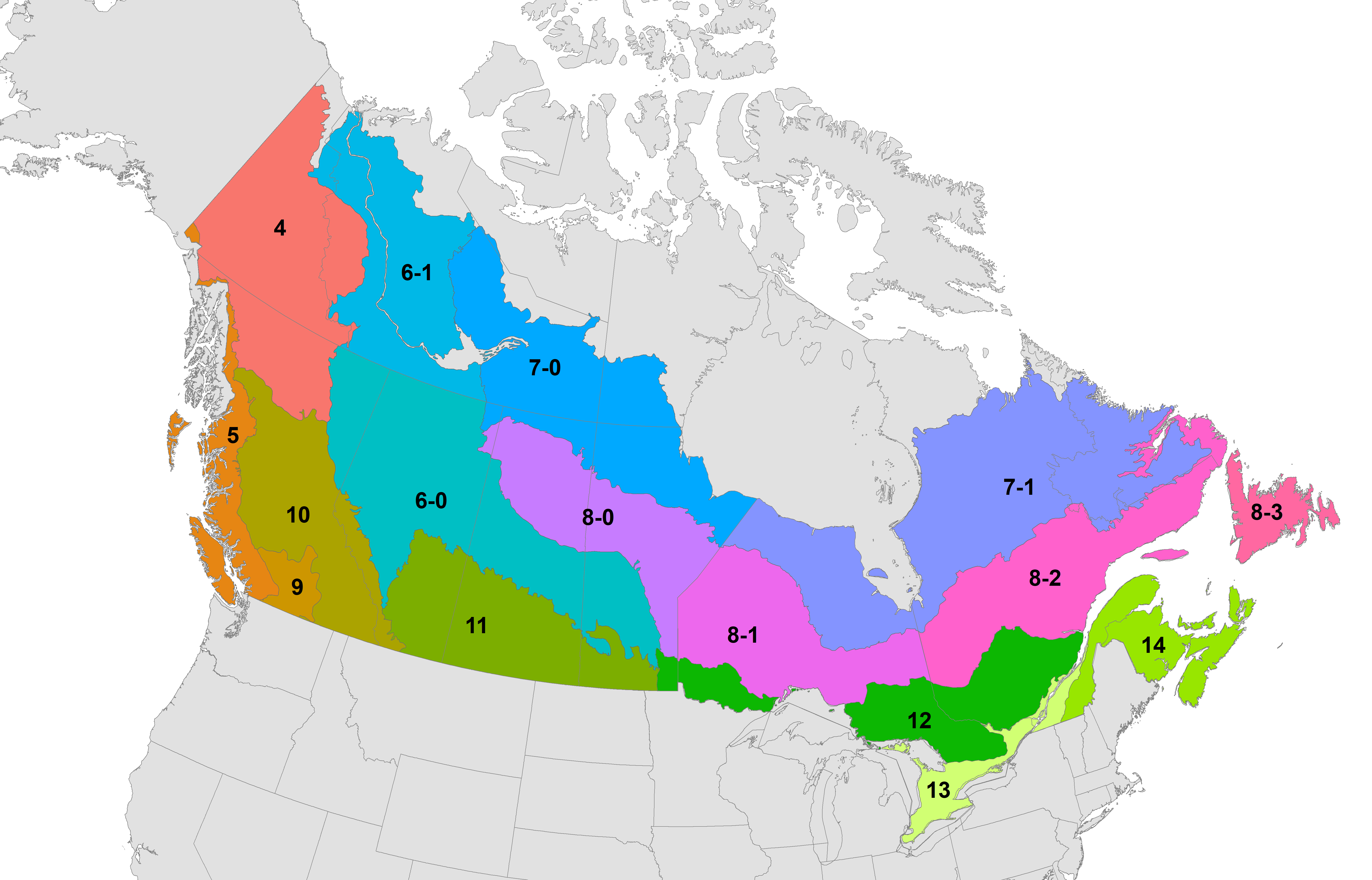
Separate models were constructed for each of 16 separate spatial subunits consisting of bird conservation regions (BCRs) intersected with Canadian jurisdictional boundaries. Smaller BCR x jurisdiction intersections were merged to maintain adequate sample sizes.

Avian data and subsampling

Avian data were extracted from the BAM avian dataset (v. 4) and supplemented with automated recording unit (ARU) data from the WildTrax acoustic database (6,801 surveys between 2012 and 2018). In total, we sampled data from 296,061 point counts across Canada (across a total of 256,316 site locations and 175 distinct projects). North American Breeding Bird Survey and provincial Breeding Bird Atlas data were included in this database, and constitute a significant fraction of available data (30% and 53% respectively).

We present models for 143 landbird species for which density offsets were available and for which data were sufficient to fit cross-validated BRTs in at least one of the 16 regions. Point-count surveys were conducted between 1991 and 2018 (97% of the point counts were from between 1997 and 2014). We stratified samples by year and geography to produce a more spatially and temporally balanced dataset. We used a 2.5 km x 2.5 km resolution spatial grid to define spatial ‘clusters’ of data. We resampled the data set in each region so that we had a single data point from each cluster/year combination and fit BRTs to the resampled data set. This subsampling addressed instances where multiple visits to the same location occurred within the same year. The subsampling was repeated 32 times.

Density calibration, detectability offsets

We accounted for differences in sampling protocol and covariate effects on detectability using statistical offsets. This included the effects of time of day and day of year on the probability of availability given presence, and the effects of tree cover and land-cover type on the probability of detection given availability (Sólymos et al. 2013). Offsets were calculated based on removal and distance-sampling models (Sólymos 2016, Sólymos et al. 2018). These models were used to predict availability and detectability for each species given survey-specific covariates. The adjustments appeared as offsets in the BRTs so that expected values represented species density.

We assumed that ARU detectability is similar to detectability by human observers (Yip et al. 2017). Nevertheless, we used an indicator variable to account for possible differences in effective area sampled between human counts and ARUs following Van Wilgenburg at el. (2017).

Environmental covariates

Model inputs consisted of 219 spatially explicit environmental covariates, as well as survey year (continuous) and survey type (binary).

To capture the influence of changing landscape conditions on avian density, we used vegetation maps from 2001 and 2011 (Beaudoin et al. 2014) and associated our survey data with the layer that represented the closest time period. Surveys conducted in 2005 or earlier were associated with the 2001 dataset, while surveys from 2006 and later were associated with the 2011 dataset. Vegetation variables were derived at a 250-m spatial resolution from k-nearest-neighbor (kNN) models that used forest sample plots from Canada’s National Forest Inventory combined with MODIS satellite imagery, as well as climate and terrain data (Beaudoin et al. 2014). Vegetation variables included pixel-level and landscape-level biomass of individual tree species and stand age. Landscape-level covariates were calculated using the focal function in the raster package for R, and were based on a moving-window average using a Gaussian weighting of surrounding pixels (one standard deviation = 750 m).

To capture other sources of landscape variation not represented in vegetation data, we supplemented the biomass and stand age covariates with several terrain, land use, and climate variables. Terrain metrics, calculated using the terrain function in the raster package for R were based on a 100-m digital elevation model for North America. Land-use and landcover variables were based on the 2005 MODIS-based 250-m North American landcover map (Commission for Environmental Cooperation). A binary (0/1) 1-km road variable (Venter et al. 2016) was used to account for the influence of roads at a broad scale. Climate variables were based on a 1-km Climate NA interpolation of 1981-2010 weather station data (Wang et al. 2016).

We pre-screened the environmental predictor variables to eliminate constant (no variation in a BCR subunit) or highly correlated (Pearson’s correlation > 0.9) variables. We also eliminated variables that never entered the cross-validated BRTs to further narrow the variable set for bootstrap to boost computing speed.

Model building

Separate models were constructed for each BCR subunit plus a 100-km buffer around the Canadian portion of the perimeter. We implemented boosted regression tree (BRT) models using the gbm.step function in the dismo R package with a Poisson distribution and 10-fold cross-validation in a preliminary run to assess the number of boosting iterations required to avoid over-fitting. We capped the number of iterations (trees) at 10,000 maximum. BRT settings were as recommended by Elith et al. (2008) and were consistent with Stralberg et al. (2015). We used the number of trees established based on the cross-validation to run models for each bootstrap sample using the gbm function in the gbm R package. This yielded 32 BRT outputs per species and subregions. We provide information on variable importance for each species by subunits, and for Canada as an average across the subunits. The top ranking variables with respect to variable importance were year of survey, temperature difference, average summer temperature, summer and annual heat/moisture index, and the proportion of developed areas, black spruce, and aspen.

Model validation

We calculated validation metrics using the training data set by making 32 predictions given the bootstrap based BRT outputs. Scale and location shifts across bootstrap based predictions were evaluated by the overall concordance correlation coefficient (OCCC; Lin 1980, Barnhart et al. 2002). OCCC measures the deviation from 1:1 line through the origin, i.e. perfect agreement between two measures. OCCC is the product of two the overall precision (how far each observation deviated from the best fit line), and the overall accuracy (how far the best line deviates from the 1:1 line).

We used the bootstrap averaged predictions to calculate expected values under the null model [exp(initial intercept estimate of the BRT + offsets)] and the final BRT [estimate from all trees combined x exp(offset)]. These initial and final predictions were used to calculate AUC (initial and final) to assess classification accuracy (counts treated as detection / non-detection) and pseudo R2 to quantify the proportion of variance explained (based on Poisson density based deviance relative to the null and saturated models).

Bootstrap averaging and prediction

We used the subregional BRT results to make species and subregion specific predictions using 1 km² resolution raster layers as predictors. Our predictions represent the expected number of male individuals per ha area given off-road habitat and human observers. We generated 32 predictions for each species x subregion combination. When the actual bootstrap sample did not contain any detections of the species we predicted 0. For each species, we mosaiced together the 16 subregion predictions for a bootstrap run (runs were independent across regions). We varied the width of the overlap zone between subregions (0-100 km) to smooth the predictions at the edges of the subregions and to avoid banded patterns. The random buffer was based on the cumulative density of the Beta(2, 2) distribution. We then averaged the 32 mosaiced layers to get the bootstrap mean of the predictions.

Density maps

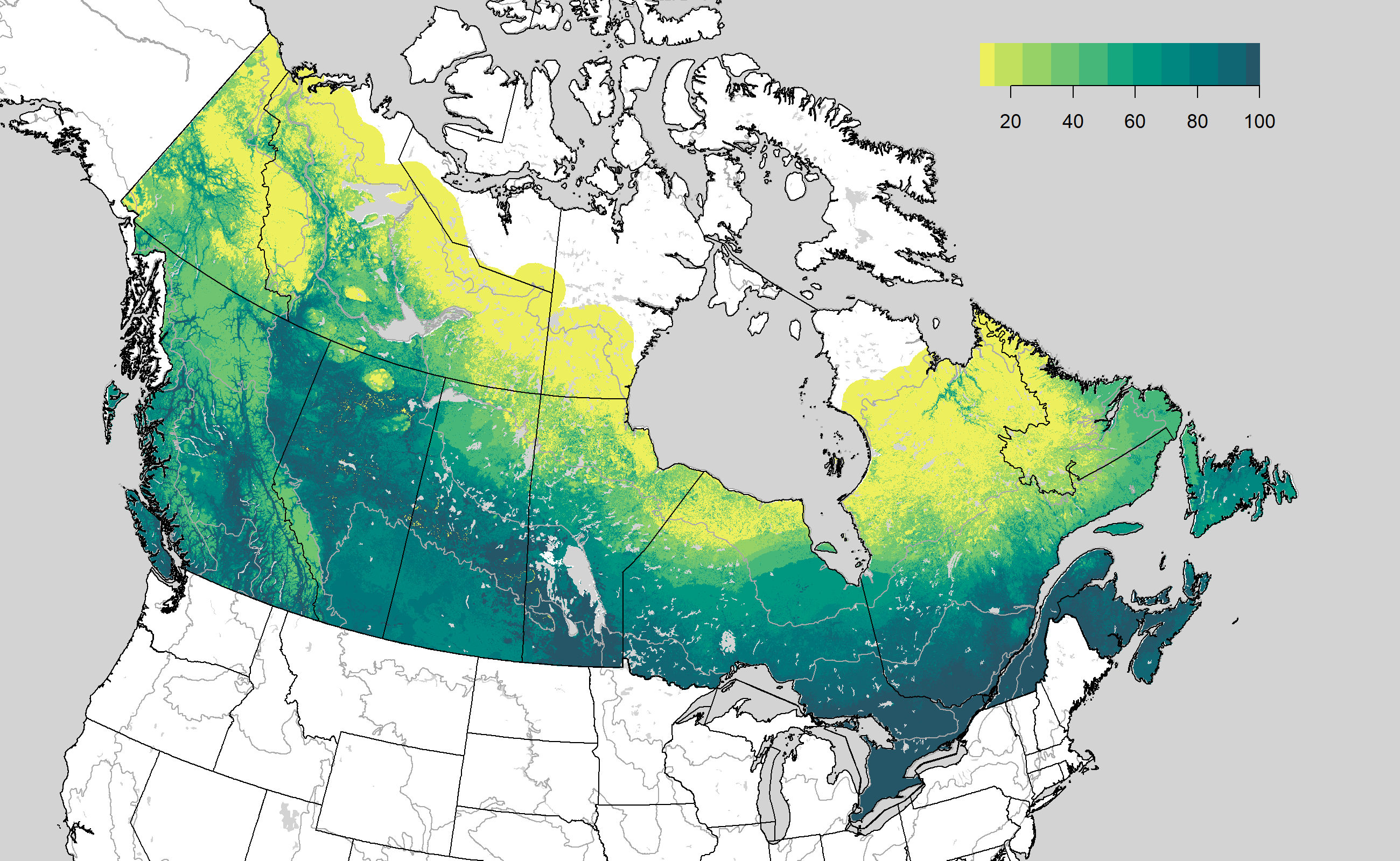
We developed separate models for each BCR subunit to improve local prediction accuracy and avoid out-of-range prediction. However, this resulted in some sharp transitions in predictions across certain boundaries that coincide with large regional differences in density. This variation in density across a large study area presented challenges for mapping, and we had to balance mapping detail with aesthetics to produce meaningful national maps. We emphasize that categorical map legends necessarily introduce subjectivity into the interpretation of species’ distribution and abundance patterns, and note that the legend breaks we used may not be the best ones for any particular mapping need. We encourage users to download the raster predictions and develop their own maps for regional applications.

Based on previous work, we started by developing maps that used mean density (males/ha) within the model-building area (Stralberg et al. 2015) as a presence/absence threshold, with areas of density below this mean density (“absence”) represented in light yellow. However, we found that this did not adequately describe the abundance patterns of all species, especially those that are widely distributed. So we adjusted the minimum thresholds according to visual alignment with known range limits. If maps based on these mean density thresholds resulted in a non-trivial number of occurrence locations mapped as absence (light yellow), then we sequentially adjusted these thresholds downward until that was no longer the case (starting with 0.05, then 0.01, then 0.001). 0.001 males/ha was the lowest density that we allowed to be used for this lower density threshold. Equal-interval legends, capped at the 99th percentile of predictions, were used to classify remaining density predictions for mapping.

The trade-off to this mapping approach is that there is perceived "over-prediction" in non-range areas (usually in the north, and often only in some BCRs). In some cases this may be related to range map inaccuracies in northern regions, but it also has to do with the sparsity of data in the north and the model's inability to identify covariates that control presence/absence. Additional data are needed to map northern range limits more accurately.

Regional population estimates

Regional population estimates (millions of male individuals) for each species and regions (Canada and subunits) were estimated by summing up the pixel level predictions within the region of interest accounting for the area difference (ha to km²). Uncertainty around the population estimates was based on the 5th and 95th percentiles of the bootstrap distribution.

Land cover based density estimates

We used a post-hoc stratification (‘post-stratification’) approach to estimate land cover based density estimates (males per ha) for each species and regions (Canada and subunits). We classified the predictive maps according to the 2005 MODIS-based North American landcover map into major land cover types (Conifer, Taiga Conifer, Deciduous, Mixedwood, Shrub, Grass, Arctic Shrub, Arctic Grass, Wetland, Cropland) and calculated the mean of the pixel level predicted densities. Uncertainty was based on the 5th and 95th percentiles of the bootstrap distribution.

Data availability

• Source code for the methodology is available on GitHub.
• Download average density raster layers in GeoTIFF format.
• Download results in Excel (xlsx) format. Sheets contain abundance and density estimates and also the list of species, variables, variable importance and validation metrics.
• Access the population size and density estimates via the JSON API.

Citing these results

Boreal Avian Modelling Project, 2020. BAM Generalized National Models Documentation, Version 4.0. Available at https://borealbirds.github.io/. DOI: 10.5281/zenodo.4018335.